Bounding Box Visualizer

Section 21.2.1

Purpose

Visualize the bounding-box sizes in your training dataset before calculating custom anchors. The scatterplot makes it easier to identify possible groups of box sizes.

Section 21.2.2

Why It Exists

It can be difficult to judge how many anchors may be appropriate without first seeing the distribution of bounding-box sizes. This utility provides that visual starting point; it does not calculate anchors or select an anchor count for you.

Section 21.2.3

Input

Use an exported YOLO / Darknet training dataset with clip folders containing images and labels subfolders. All images must have the same resolution.

Annotations contain five whitespace-separated numbers per object:

class_id  center_x  center_y  width  height
0         0.50      0.50      0.25   0.20

The script searches recursively through folders named labels, combines their boxes, and obtains the image resolution from the first readable PNG, JPG, or JPEG image. It ignores empty label files and skips lines without exactly five values.

Section 21.2.4

Output

One figure contains two side-by-side plots: bounding-box width versus height, and a 20-bin histogram of bounding-box areas. Each point represents a labeled box; the histogram counts boxes by area.

Configuration anchors are based solely on bounding-box size, regardless of class name. Visualizing box sizes is a critical step in building custom configurations.

Pixel dimensions

The default view plots width and height in pixels, and area in square pixels. Read the axis values before judging how different the box sizes are.

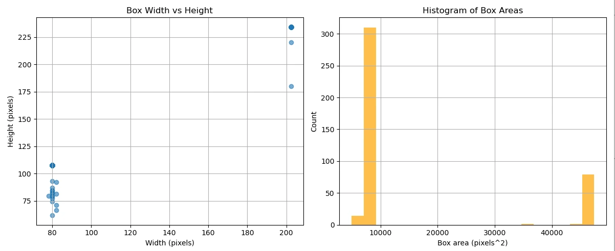
Relative dimensions

With --scaled, width and height are fractions of the image dimensions, and area is a fraction of the full image area. The scatterplot axes span 0 to 1. The underlying box-size relationships remain unchanged.

Review both views in sequence for two perspectives on the same data. Close the first plot window before running the second command.

Section 21.2.5

How To Use

Save bounding_box_visualizer.py in the main project folder, alongside your clip folders. Prepare the virtual environment and install NumPy, Matplotlib, and OpenCV using 21.1 · Python & Libraries.

Choose your system. These commands assume the project environment is named .venv.

source .venv/bin/activate

python bounding_box_visualizer.py .

python bounding_box_visualizer.py . --scaled

.venv\Scripts\activate.bat

python bounding_box_visualizer.py .

python bounding_box_visualizer.py . --scaled

If something goes wrong

• No valid image: confirm that the dataset contains a readable PNG, JPG, or JPEG.
• No usable boxes: confirm that lowercase labels folders contain non-empty .txt files with five numeric values per box.
• Missing package: activate your project’s virtual environment, then install the missing package using python -m pip install package-name. Replace package-name with the required package name; for example, the cv2 module is provided by opencv-python.
• No plot window: run in a desktop session capable of displaying Matplotlib windows.

The script reads the dataset and displays plots; it does not modify annotations or write plot files automatically.

Section 21.2.6

Code

The complete program from section 21.2, with PDF line wrapping and indentation restored for use as a Python file.

import os
import sys
import cv2
import numpy as np
import argparse
import matplotlib.pyplot as plt


def get_image_resolution(dataset_path):
    for root, dirs, files in os.walk(dataset_path):
        for file in files:
            if file.lower().endswith((".png", ".jpg", ".jpeg")):
                img_path = os.path.join(root, file)
                img = cv2.imread(img_path)
                if img is not None:
                    height, width = img.shape[:2]
                    return width, height
    raise ValueError("No valid image file found to determine resolution.")


def extract_wh_from_label(label_path, img_w, img_h):
    wh_list = []
    with open(label_path, "r") as f:
        for line in f:
            parts = line.strip().split()
            if len(parts) != 5:
                continue
            _, _, _, w, h = map(float, parts)
            abs_w = w * img_w
            abs_h = h * img_h
            wh_list.append([abs_w, abs_h])
    return wh_list


def collect_boxes(dataset_path, use_scaled=False):
    wh_data = []
    img_w, img_h = get_image_resolution(dataset_path)
    for root, dirs, files in os.walk(dataset_path):
        if os.path.basename(root) == "labels":
            for file in files:
                if file.endswith(".txt"):
                    label_path = os.path.join(root, file)
                    if os.path.getsize(label_path) == 0:
                        continue
                    wh = extract_wh_from_label(label_path, img_w, img_h)
                    if use_scaled:
                        # Convert to fraction of image dimensions
                        wh = [[w / img_w, h / img_h] for w, h in wh]
                    wh_data.extend(wh)
    if not wh_data:
        raise ValueError("No non-empty label files found in the dataset.")
    return np.array(wh_data, dtype=np.float32), img_w, img_h


def visualize_boxes(boxes, img_w, img_h, use_scaled=False):
    widths = boxes[:, 0]
    heights = boxes[:, 1]
    areas = widths * heights
    plt.figure(figsize=(12, 5))
    # Scatter plot of width vs height
    plt.subplot(1, 2, 1)
    plt.scatter(widths, heights, alpha=0.6)
    if use_scaled:
        plt.xlim(0, 1)
        plt.ylim(0, 1)
        plt.xlabel("Width (fraction of image width)")
        plt.ylabel("Height (fraction of image height)")
        plt.title("Box Size Relative to Image Dimensions")
    else:
        plt.xlabel("Width (pixels)")
        plt.ylabel("Height (pixels)")
        plt.title("Box Width vs Height")
    plt.grid(True)
    # Histogram of box areas
    plt.subplot(1, 2, 2)
    plt.hist(areas, bins=20, color='orange', alpha=0.7)
    if use_scaled:
        plt.xlabel("Box area (fraction of image area)")
        plt.title("Histogram of Box Areas (Relative)")
    else:
        plt.xlabel("Box area (pixels^2)")
        plt.title("Histogram of Box Areas")
    plt.ylabel("Count")
    plt.grid(True)
    plt.tight_layout()
    plt.show()


if __name__ == "__main__":
    parser = argparse.ArgumentParser(
        description="Visualize the distinct box sizes in a YOLO dataset."
    )
    parser.add_argument(
        "dataset_path",
        type=str,
        help="Path to dataset directory (must contain a 'labels' folder)."
    )
    parser.add_argument(
        "--scaled",
        action="store_true",
        help="Use relative image dimensions (0–1 scale) instead of absolute pixel sizes"
    )
    if len(sys.argv) == 1:
        parser.print_help(sys.stderr)
        sys.exit(1)
    args = parser.parse_args()
    boxes, img_w, img_h = collect_boxes(args.dataset_path, args.scaled)
    visualize_boxes(boxes, img_w, img_h, args.scaled)

Section 21.2.7

Prompt to Reproduce This Utility with AI

Copy the complete request below into your AI chat. Review and test any generated code before using it.

Replace [your favorite programming language] at the top of the request with the language you want the AI to use. The downloadable code and How To Use instructions on this page remain the book’s Python version.

Programming language: [your favorite programming language]

Create a complete program that analyzes the bounding box dimensions in a YOLO/Darknet training dataset and visualizes their size distribution.

The program will be placed in the main project folder. Beneath the project folder will be one or more clip folders. Each clip folder contains images and labels subfolders. The program must recursively search all clip folders, read every valid label file and combine the bounding boxes from the entire dataset into a single set of results.

The annotation files use the standard YOLO/Darknet format, with five whitespace-separated values per object:

class_id  center_x  center_y  width  height

The coordinates and dimensions are normalized between 0 and 1. Convert the normalized width and height values to pixel dimensions using the image resolution. Assume all images in the dataset have the same resolution and determine that resolution from the first valid .png, .jpg or .jpeg image found in the dataset.

Ignore empty label files and skip annotation lines that do not contain exactly five values.

Generate a single figure containing two side-by-side plots:
- A scatterplot showing bounding box width versus bounding box height
- A histogram showing the frequency distribution of bounding box areas

By default, display the results using absolute pixel dimensions. Add an optional --scaled command-line flag that instead displays bounding box width and height normalized between 0 and 1 relative to the image dimensions. The histogram should also display normalized box areas.

The program should be executable from the terminal. Provide build or setup instructions, required dependencies, and commands appropriate to the chosen language for running the program against the current project folder, represented by a single dot, both with and without the --scaled flag. The program should automatically process the entire dataset and produce a single figure representing all clip folders. Use suitable libraries for image loading, numerical processing, plotting, and command-line argument parsing.