
Section 21.3.1
Purpose
Visualize the relationship between labeled objects and the detection-layer grids you are considering for your configuration. This is the chapter’s second step in evaluating detection-layer requirements.
The utility is not required to calculate custom anchors. Reviewing stride alongside bounding-box sizes helps you consider both box size and spatial arrangement.
Section 21.3.2
Why It Exists
Overlaying stride-32, stride-16, and stride-8 grids makes it easier to judge how closely spaced object centers relate to grid cells. It provides a visual reference while you develop the ability to picture these grids mentally.
The book explains that with experience, the author no longer needs this utility to visualize the grids. For a newcomer, the overlays make that relationship tangible.
Section 21.3.3
Input
Use an exported YOLO / Darknet training dataset. Place the script in the project folder, alongside the clip folders. Each clip must have lowercase images and labels subfolders, with matching image and annotation filename stems.
Unlike the recursive box-size collector in 21.3, this script examines clip folders directly beneath the supplied project folder. Clip folders and image filenames are processed in sorted order.
class_id  center_x  center_y  width  height
0         0.50      0.50      0.25   0.20
Annotations use normalized coordinates. The program converts them to box corners using the resized image dimensions. It supports PNG, JPG, and JPEG images, skips unreadable images, and skips annotation lines that do not contain five values. Five-value lines must be numeric.
Review 21.1 · Data Structure & Python Setup →Section 21.3.4
Output
Each image is resized to the requested network resolution and displayed with its labeled boxes in green and the selected stride grid overlaid. A few representative images are often enough to assess the arrangement.
| Head | Stride | Grid at 416 × 416 | Grid color |
|---|---|---|---|
| 1 | 32 | 13 × 13 | Red |
| 2 | 16 | 26 × 26 | Blue |
| 3 | 8 | 52 × 52 | Yellow |
These head numbers belong to this utility. Other software may number or order detection heads differently.
Stride 32 · larger objects
Each nut’s bounding-box center falls in a different grid cell. This is a favorable spatial arrangement, provided the objects are also large and visually distinct enough for that detection scale.

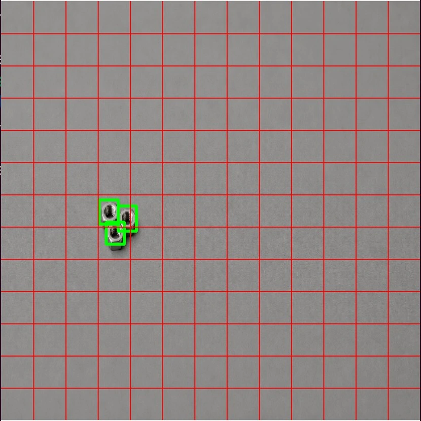
Stride 32 · smaller, closely spaced objects
With the same 13 × 13 grid, two small nut centers fall in the same cell and the third is nearby. This can make learning and detection more difficult at this stride, particularly when similar objects compete for the same anchors.
Stride 8 · the same small objects
The finer 52 × 52 grid places each nut center in a different cell. The book identifies stride 8 as the likely better choice for these small, closely spaced nuts.

A favorable arrangement is not a guarantee of detection performance. Consider object size, spacing, visual detail, and your actual model’s behavior together.
Section 21.3.5
How To Use
Save grid_stride_visualizer.py in the project folder. Use the setup in 21.1 · Python & Libraries to create the project environment. This utility needs opencv-python; os and argparse are included with Python.
Linux Terminal
Open a terminal in the project folder and activate the environment:
source .venv/bin/activateInstall the required package if it is missing:
python -m pip install opencv-pythonRun one of the following commands. Exit the current run before choosing another head:
python grid_stride_visualizer.py . --net_w 416 --net_h 416 --head 1
python grid_stride_visualizer.py . --net_w 416 --net_h 416 --head 2
python grid_stride_visualizer.py . --net_w 416 --net_h 416 --head 3
Inside the activated environment, python runs its Python 3 interpreter on Linux.
Windows Command Prompt
Open Command Prompt in the project folder and activate the environment:
.venv\Scripts\activate.batInstall the required package if it is missing:
python -m pip install opencv-pythonRun one of the following commands. Exit the current run before choosing another head:
python grid_stride_visualizer.py . --net_w 416 --net_h 416 --head 1
python grid_stride_visualizer.py . --net_w 416 --net_h 416 --head 2
python grid_stride_visualizer.py . --net_w 416 --net_h 416 --head 3
Inside the activated environment, python runs its Python 3 interpreter on Windows.
Controls and options
- Any key: with an image window focused, advance to the next image.
- Escape: exit immediately and close all image windows.
- Dataset path:
.means the current project folder. Replace it with another path if needed; quote paths containing spaces. - --head: required; use 1, 2, or 3.
- --net_w and --net_h: default to 416 when omitted. Use your intended network dimensions and dimensions divisible by the selected stride.
The code resizes directly to the requested network dimensions. If the source and network aspect ratios differ, the image and objects appear stretched. This is not a letterbox or padding preview.
If something goes wrong
- No images displayed: check that the supplied project folder directly contains clip folders with both
imagesandlabelssubfolders. - Grid but no boxes: check for a matching
.txtlabel file. A missing file does not prevent the image and grid from displaying. - Missing package: activate the project environment and install the missing dependency. The
cv2module comes fromopencv-python. - No display window: use a desktop session and the desktop OpenCV package, rather than its headless variant.
The program displays overlays without modifying your source images or annotations. It does not save the overlaid images.
Section 21.3.6
Code
The complete program from section 21.3, with PDF line wrapping and indentation restored for use as a Python file.
import os
import cv2
import argparse

# YOLO head strides
YOLO_STRIDES = {
    1: 32,  # Head 1
    2: 16,  # Head 2
    3: 8,   # Head 3
}

# Colors per head (OpenCV uses BGR)
HEAD_COLORS = {
    1: (0, 0, 255),     # Red
    2: (255, 0, 0),     # Blue
    3: (0, 255, 255),   # Yellow
}


def draw_grid(img, grid_w, grid_h, color=(0, 255, 255)):
    h, w = img.shape[:2]
    step_x = w / grid_w
    step_y = h / grid_h
    for i in range(1, grid_w):
        x = int(i * step_x)
        cv2.line(img, (x, 0), (x, h), color, 1)
    for j in range(1, grid_h):
        y = int(j * step_y)
        cv2.line(img, (0, y), (w, y), color, 1)


def draw_boxes(img, label_path):
    h, w = img.shape[:2]
    if not os.path.exists(label_path):
        return
    with open(label_path, "r") as f:
        for line in f:
            parts = line.strip().split()
            if len(parts) != 5:
                continue
            _, cx, cy, bw, bh = map(float, parts)
            x1 = int((cx - bw / 2) * w)
            y1 = int((cy - bh / 2) * h)
            x2 = int((cx + bw / 2) * w)
            y2 = int((cy + bh / 2) * h)
            cv2.rectangle(img, (x1, y1), (x2, y2), (0, 255, 0), 2)


def view_dataset(dataset_root, head, net_w, net_h):
    if head not in YOLO_STRIDES:
        raise ValueError(f"Invalid head: {head}. Must be 1, 2, or 3.")
    stride = YOLO_STRIDES[head]
    grid_w = net_w // stride
    grid_h = net_h // stride
    color = HEAD_COLORS[head]
    # Loop through all subfolders (each should be a dataset)
    for folder_name in sorted(os.listdir(dataset_root)):
        dataset_path = os.path.join(dataset_root, folder_name)
        if not os.path.isdir(dataset_path):
            continue
        images_dir = os.path.join(dataset_path, "images")
        labels_dir = os.path.join(dataset_path, "labels")
        if not os.path.isdir(images_dir) or not os.path.isdir(labels_dir):
            continue  # Skip folders that aren't YOLO datasets
        print(f"\nViewing dataset: {folder_name}")
        image_files = sorted(
            f for f in os.listdir(images_dir)
            if f.lower().endswith((".jpg", ".jpeg", ".png"))
        )
        for img_name in image_files:
            img_path = os.path.join(images_dir, img_name)
            label_path = os.path.join(
                labels_dir, os.path.splitext(img_name)[0] + ".txt"
            )
            img = cv2.imread(img_path)
            if img is None:
                continue
            img_resized = cv2.resize(img, (net_w, net_h))
            draw_boxes(img_resized, label_path)
            draw_grid(img_resized, grid_w, grid_h, color=color)
            window_label = f"{folder_name} | Head {head} Grid {grid_w} x{grid_h}"
            cv2.imshow(window_label, img_resized)
            key = cv2.waitKey(0)
            if key == 27:  # ESC
                cv2.destroyAllWindows()
                return
    cv2.destroyAllWindows()


if __name__ == "__main__":
    parser = argparse.ArgumentParser(
        description="Visualize YOLO grid for a given head and network resolution"
    )
    parser.add_argument("dataset_path", type=str, help="Path to YOLO dataset root")
    parser.add_argument(
        "--head", type=int, choices=[1, 2, 3], required=True,
        help="YOLO head (1, 2, or 3)"
    )
    parser.add_argument("--net_w", type=int, default=416, help="Network width")
    parser.add_argument("--net_h", type=int, default=416, help="Network height")
    args = parser.parse_args()
    view_dataset(args.dataset_path, args.head, args.net_w, args.net_h)
Section 21.3.7
Prompt to Reproduce This Utility with AI
Copy the complete request below into your AI chat. Review and test any generated code before using it.
Replace [your favorite programming language] at the top of the request with the language you want the AI to use. The downloadable code and How To Use instructions on this page remain the book’s Python version.
Programming language: [your favorite programming language]

Create a complete program that visualizes how YOLO grid cells relate to labeled objects in a standard Darknet training dataset.

The program will be placed in the main project folder. Beneath the project folder will be one or more clip folders. Each clip folder contains images and labels subfolders. Process these clip folders in sorted order, skip folders that do not contain both required subfolders, and display every valid image one at a time in sorted filename order. Support .png, .jpg, and .jpeg images, regardless of extension case. Match each image to a .txt label file with the same filename stem.

Resize each image to a user-specified network resolution. Use 416 by 416 as the default resolution. Draw the bounding boxes from the corresponding YOLO/Darknet label file, then overlay the grid associated with the selected detection head.

Annotations contain five whitespace-separated numeric values per object:
class_id  center_x  center_y  width  height
The coordinates and dimensions are normalized. Convert them to bounding-box corners using the resized image dimensions. Draw the boxes in green.

Use this head mapping and grid colors:
- Head 1 = stride 32, red grid
- Head 2 = stride 16, blue grid
- Head 3 = stride 8, yellow grid

Calculate the grid columns as network width divided by stride using integer division, and the grid rows as network height divided by stride using integer division. Draw the internal grid boundaries. At 416 by 416, the grids are 13 by 13, 26 by 26, and 52 by 52, respectively.

Support these command-line options:
- A positional dataset_path argument for the project folder
- --head, required, accepting 1, 2, or 3
- --net_w, network width, default 416
- --net_h, network height, default 416

Display the images in a desktop window. Advance to the next image when any key is pressed. Exit immediately and close all image windows when Escape is pressed. Close all image windows when the dataset is finished.

Skip images that cannot be opened. If a matching label file is missing, still display the image and grid. Ignore annotation lines that do not contain exactly five values. Assume that five-value lines contain valid numeric annotations.

Do not modify the source images or annotations. Use suitable libraries for image loading, resizing, drawing, desktop display, filesystem access, and command-line argument parsing. Provide the complete program, dependency and setup instructions, and commands for running all three heads using the chosen language. Explain any direct-resize aspect-ratio distortion.